Data Visualization
I have included four #TidyTuesday visualizations that I have created. The code and full viz for each project can be found on my GitHub pages in the links.
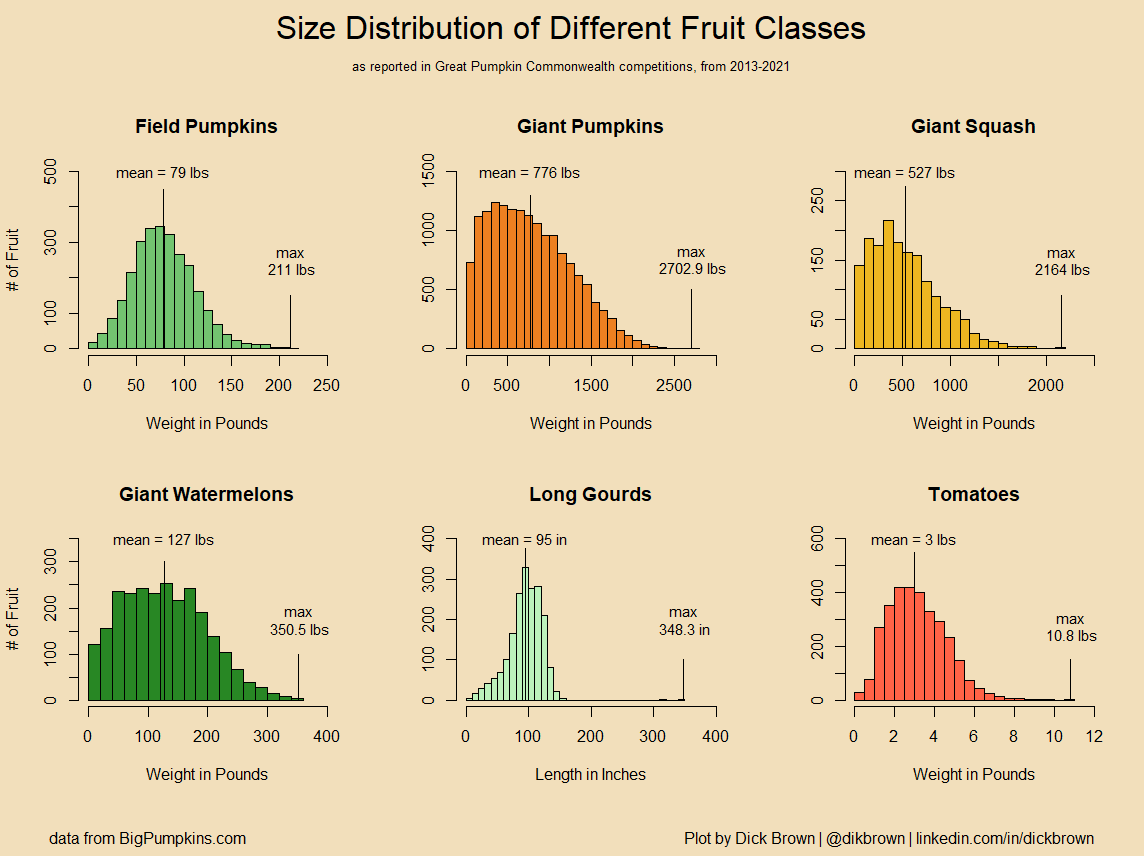
The Great Pumpkins viz was created with the base plotting functionality, using hist(). The layout was created by creating a matrix with a top panel for the viz title, two rows of three panels for the six graphs, and a bottom panel for the citation. The split.screen() function was then called with the matrix set up the different panels. Then, the screen() function was called before writing to each of the eight panels. I chose the plot colors to try to match the colors of the fruit, and the background to give it an autumn feel. The dataset was supplied by the #TidyTuesday github.
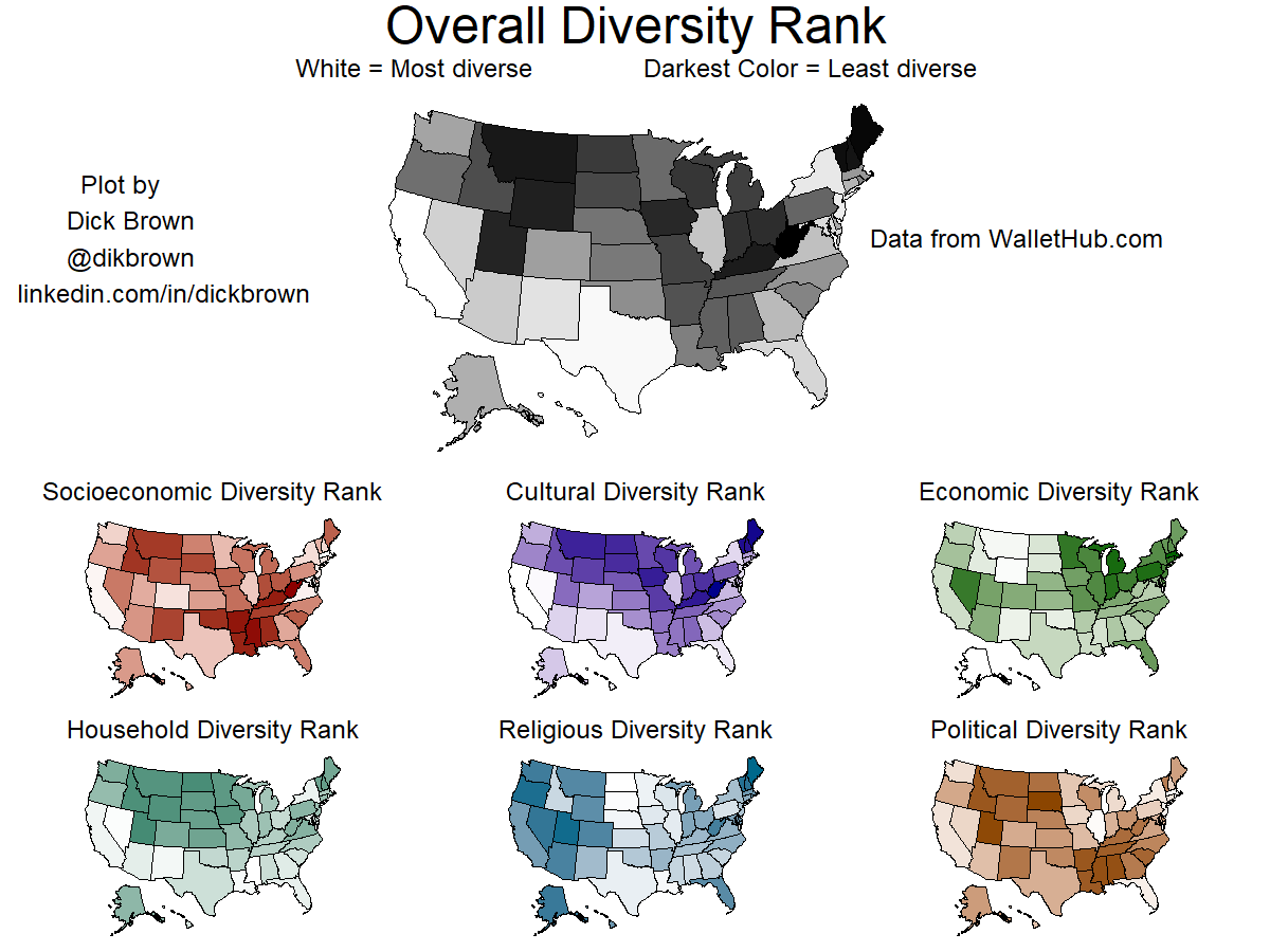
The Diversity viz was created with ggplot(). The split.screen() function does not work with the ggplot2 package, so I had to try something else. I again created a matrix to define the layout and assigned the seven maps to unique variables. I then called grid.arrange() with the textGrobs (to the left and right of the main map) and the seven variables corresponding to the seven maps. I created the dataset from tables found on Wallethub's website.
The Runners viz was created with ggplot(). I used geom_label() to place the bar labels inside the bars. The dataset was supplied by the #TidyTuesday github.
Finally, the Seafood Production viz was created with ggplot(). It's a simple stacked area plot. The complete dataset was composed of seven separate tables and was supplied by the #TidyTuesday github. I decided to work with the "fish-anad-seafood-consumption-per-capita" table. To simplify things, I decided to summarize seafood consumption by continent. Fortunately, the dataset included these values, plus the overall world values, which I included as a reference line. Although the data dictionary didn't mention this, I assume that the gap is due to small island nations that aren't included in any of the six continents.


The first three of these visualizations were created as part of contests. The last was just practice, and I can't find any record of it being posted anywhere except Tableau Public.
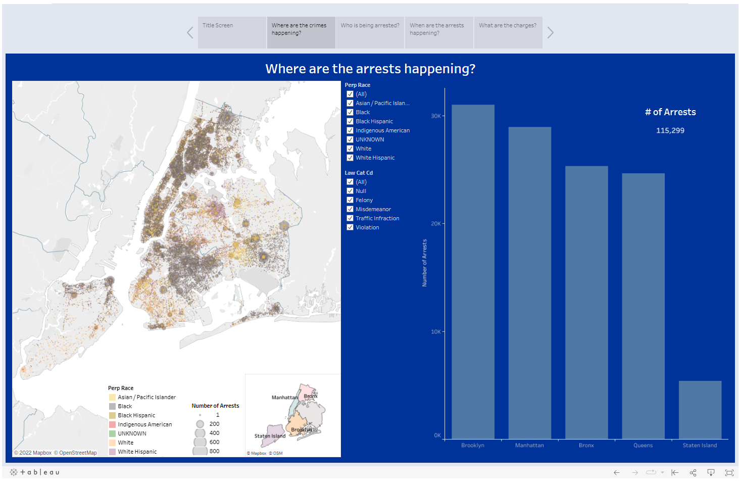
The first visualization is one page of a dashboard I created for Onyx's November 2021 Data Challenge. The dataset was provided by Onyx. The complete dashboard includes a title page plus four more pages representing the where, who, when and what of arrests in New York City in the first nine months of 2021. The picture of NYC on the title page is one I took while I was on vacation a few years ago. I think it was from the shore of Liberty Park, in New Jersey.
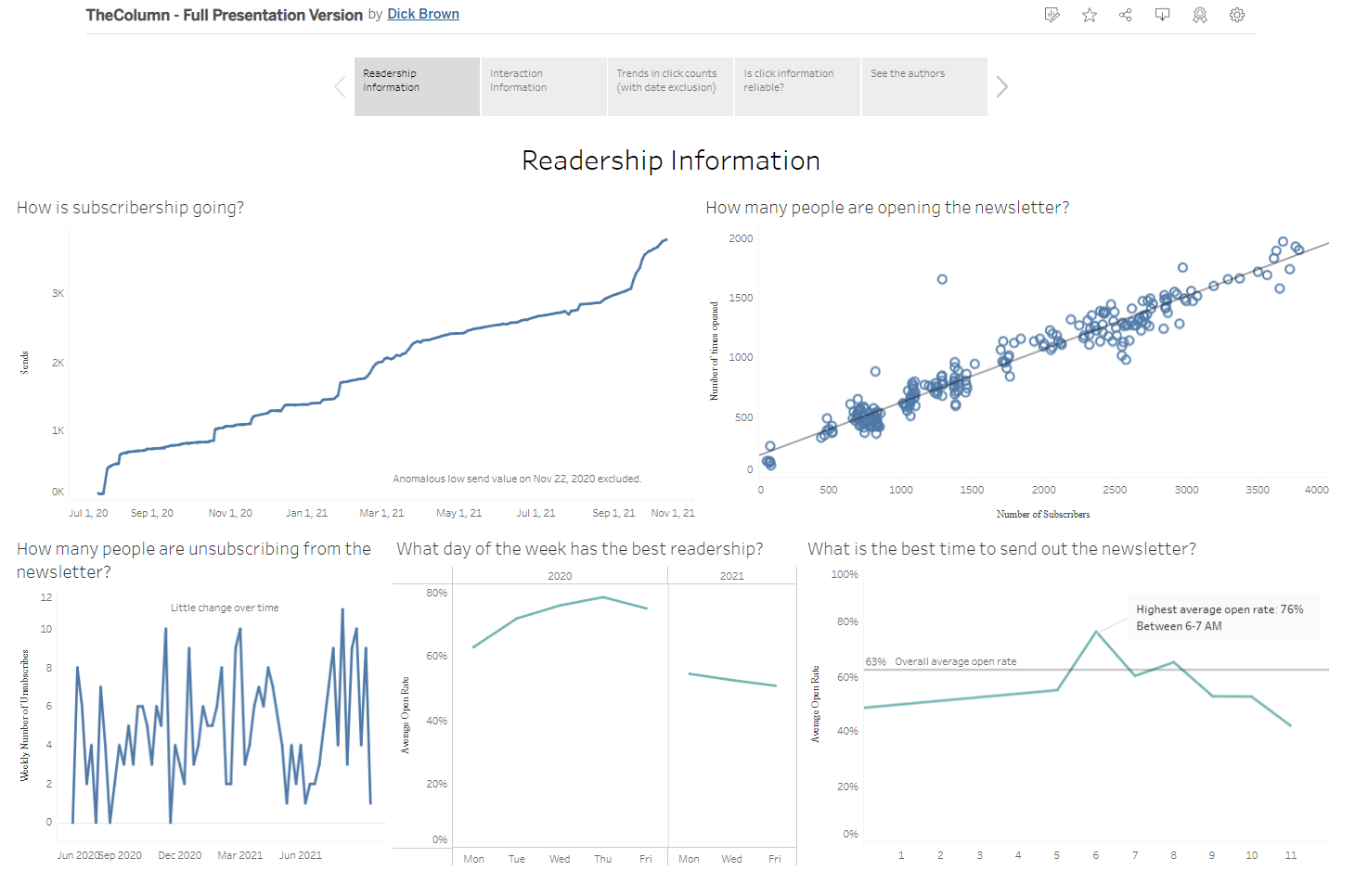
The second visualization is one page of a dashboard I created for Avery Smith's Data Career Jumpstart Hackathon, in October, 2021. I was part of the winning team in the hackathon, and the presentation we put together is shown on the Presentations page of this website. The purpose of the project was to see what information we could pull from a series of files representing readership and click information from The Column newsletter.
The third visualization was created for Onyx's February 2022 Data Challenge, although I never got around to submitting it. The dataset was provided by Onyx and represents number of travelers from the United States and what country they traveled to. This left side of this single-page dashboard compares the different destination countries in terms of number of travelers. At the top is a slider to move through time in the dataset, starting in May 1990 and going through June 2021. Red represents the "hottest" destinations. At the bottom is a bar chart ranked by number of travelers, again color-coded by number of travelers. This lets the viewer see at a glance where travel is focused. On the right side, I've got a time series showing change in travel over time. We can see here that traveled dropped a lot in the years after 2000. This was precipitated by the terrorist attacks of 9/11/2001. This can be seen more clearly in the more detailed view above the main graph, which shows a huge decline in September and October, which are usually mid-range shoulders on the large summer peak preceding the large drop in travel over the winter.
Finally, the last visualization is a new visualization from a #MakeoverMonday dataset. This was posted to Tableau Public, but for some reason, I never posted it to my Twitter or LinkedIn feed. I had posted a different viz from this dataset earlier, but wanted to try something both simpler and more creative. I didn't have much experience with Tableau at the time, and it could probably use some work.

Drop me a line and we can talk. It can be about a job, or a discussion of the website, or just the start of a beautiful friendship.